ME News

wrote a column ·

The 'Pitfalls' of Market Prediction: Why You Always Lose on Your Bets

Author: Terry Lee

Article compiled by: BitpushNews

Source: Terry's Takes

On platforms like Polymarket, most people (including my former self) typically price parlays—multiple event combo bets—by simply multiplying the probabilities of each individual event.

For example:

Probability of Event A occurring P(A) = 80%

Probability of Event B occurring P(B) = 70%

The probability of Event C occurring, P(C), is 60%.

Thus, the total probability of the parlay = 80% × 70% × 60% = 33.6%.

(Note: Parlays is a term used in gambling and investing, commonly referred to as 'parlay' or 'cross-over' in Chinese. Definition: You combine two or more independent event bets into one. Rule: You only win the payout if all selected events are predicted correctly. If any one prediction is wrong, the entire bet is lost.)

Sounds simple, right?

The problem doesn't lie in the mathematical calculation but in the hidden assumptions.

The premise of this multiplication operation assumes that each event is mutually independent. This means the outcome of A has no effect on B. However, in reality, this is often not the case.

For example:

The Federal Reserve's decision at a particular meeting can significantly impact the next meeting.

A presidential candidate winning the 'Rust Belt' states indicates a higher likelihood of success in Pennsylvania, further influencing the overall chances of winning the presidential election.

In reality, the vast majority of events worth creating parlays for are interconnected. If you overlook this interdependence, you may end up overpaying or missing out on profitable opportunities.

This article will present a simple framework to teach you how to scientifically price parlays, similar to how traditional finance has priced multi-leg options for decades.

In my view, the majority ofPrediction marketstools focus on 'execution' rather than 'correlation analysis.' Moreover, this niche market is still relatively immature. While 'parlay betting' is common in sports gambling, when dealing with specific social/economic events, pricing mechanisms remain underdeveloped due to the market's early stage.

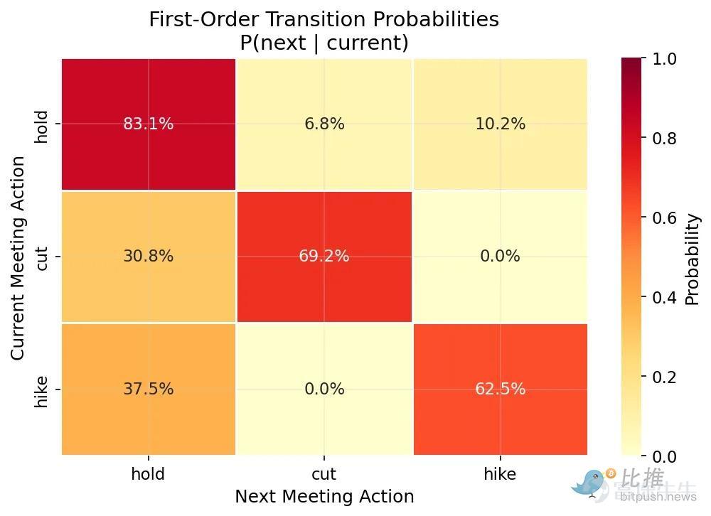
(Figure 1: The Federal Reserve tends to repeat actions, maintaining interest rates again 83% of the time after initially 'maintaining'.)

Using data from the St. Louis Fed (FRED) spanning from 1994 to early 2026, I constructed a transition matrix specifically extracting the Federal Reserve’s decision changes between consecutive meetings.

The results are very clear:

Maintain -> Maintain: Probability of 83.1%

Rate cut -> Rate cut: Probability of 69.2%

Rate hike -> Rate hike: Probability of 62.5%

Clearly, the Federal Reserve operates with 'continuity.' As a forward-looking, data-dependent institution, they tend to repeat the same action until there is a 'regime shift.'

To test this, I built a model to identify every historical instance of 'decision trends' (i.e., each consecutive cycle of maintaining, cutting, or raising rates).

The results are as follows:

Maintaining interest rates: A total of 32 trends observed, averaging 5.4 meetings per trend.

Rate cuts: A total of 12 trends observed, with an average duration of 3.3 meetings per trend.

Next, I simulated the Federal Reserve's history across 1,000 'parallel universes.' In these simulations, each meeting was independent (similar to flipping a coin). Based on historical aggregate data, the probability of maintaining rates was set at 66%, rate cuts at 15%, and rate hikes at 19%, with no correlation between decisions.

(Figure 2: The actual decision coherence of the Federal Reserve is 2-3 times higher than random probability)

Under the assumption of 'mutual independence' in the simulation, the trend of maintaining interest rates lasted an average of only 2.9 meetings, while rate cuts and rate hikes averaged just 1.2 meetings.

Comparing actual history with random simulations:

Maintain: Actual 5.4 vs Random 2.9 (1.9 times longer)

Rate cuts: Actual 3.3 vs Random 1.2 (2.8 times longer)

Rate hikes: Actual 2.6 vs Random 1.2 (2.1 times longer)

Notably, the coherence of rate cuts is nearly three times higher than random probability. The reason is that when the Federal Reserve begins cutting rates, it is typically in response to ongoing economic deterioration, which cannot be resolved within a single meeting. They cut rates, assess the data, and if the data remains poor, they are highly likely to cut again.

A simple multiplication calculation for 'sequential events' completely overlooks these correlations. The coherence observed in reality is 2-3 times stronger than in an independent random model.

Looking at just the last meeting is insufficient; pricing the 'triple test' (a combination of three events) requires studying the conditional probabilities based on the outcomes of the previous two meetings.

The analysis can be divided into two parts:

(Figure 3: After two identical actions, the third action almost always matches)

As clearly shown in Figure 3, when the Federal Reserve repeats the same action twice, the probability of continuing that action for the third time is overwhelming:

Two holds -> Third hold: 87%

Two rate hikes -> Third rate hike: 84%

Two rate cuts -> Third rate cut: 68% (slightly weaker)

Also worth noting are the 0% cells in the matrix: The Federal Reserve has never suddenly cut rates after two consecutive rate hikes, nor raised rates after two consecutive rate cuts. They always go through a 'pause (hold)' phase first. Simply being aware of this can help you eliminate a range of invalid combinations that 'naive models' might consider valuable.

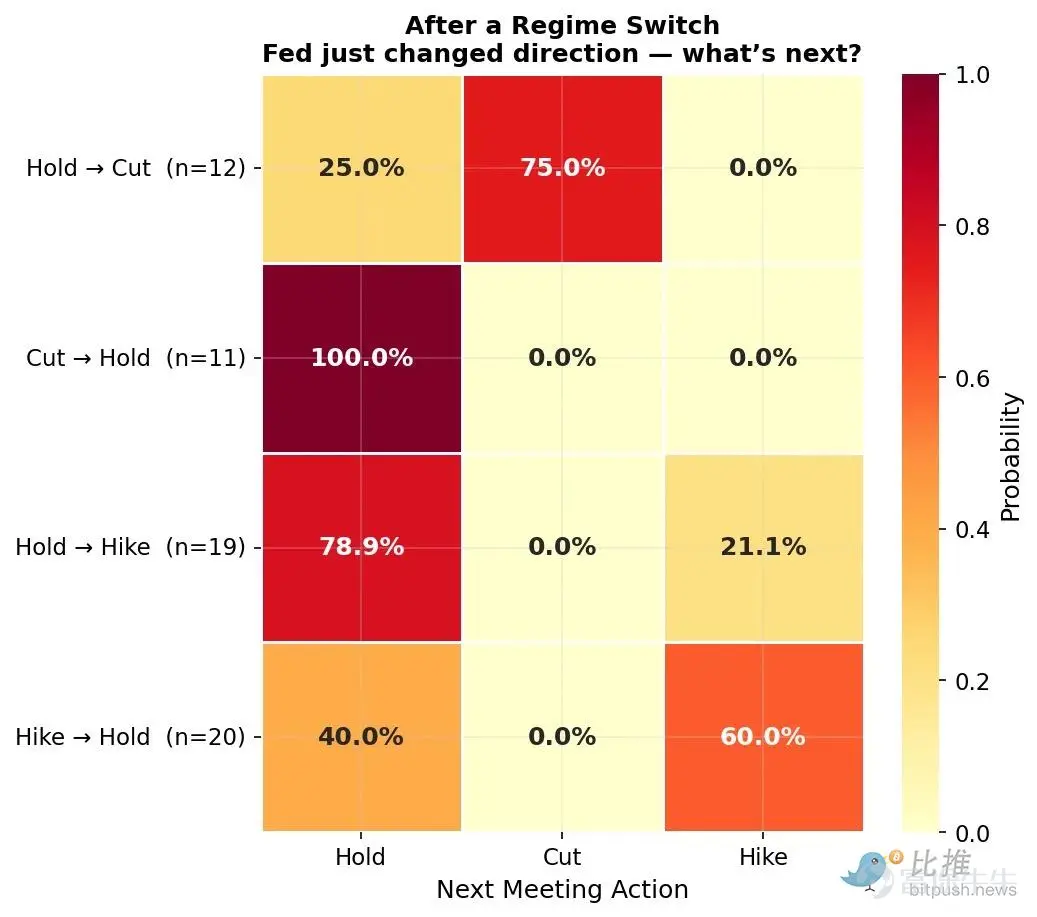
(Figure 4: The differences in directional changes after regime shifts are substantial)

This is the most interesting part for traders. Not all directional changes are equal:

Maintain -> Cut rates -> Cut rates: Probability is 75%. Once the Fed breaks the hold and begins the first rate cut, the 'floodgates' open and subsequent cuts are highly likely.

Cut rates -> Maintain -> Maintain: Probability is 100%. In recent history, the Fed has never resumed cutting immediately after pausing. A single pause means a full stop!

Maintain -> Raise rates -> Maintain: Probability is 79%. The first rate hike after a holding period tends to be tentative, as they will pause to observe the impact.

Raise rates -> Maintain -> Raise/Maintain: Probabilities are 60% and 40%, respectively. Unlike with rate cuts, pauses during a hiking cycle carry genuine uncertainty.

This asymmetry is the core insight. The combination value of 'Maintain -> Cut rates -> Cut rates' is much higher than what simple multiplication would suggest. Meanwhile, combinations like 'Cut rates -> Maintain -> Cut rates' have historically had almost no value. The same outcomes but in a different order can result in vastly different true values. Independent multiplicative models fail to capture this nuance.

This is the bigger picture. We should not use blind average probabilities but rather conditionally observed historical probabilities.

Take 'three consecutive holds (Hold-Hold-Hold)' as an example:

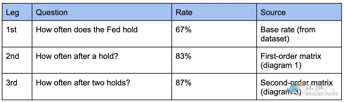
Initial model: Using overall probability (hold probability 67%), calculated as 67% × 67% × 67% = 30.1%.

Revised model: Using conditional probability, calculated as 67% (first hold) × 83% (second hold | first) × 87% (third hold | first two) = 48.4%.

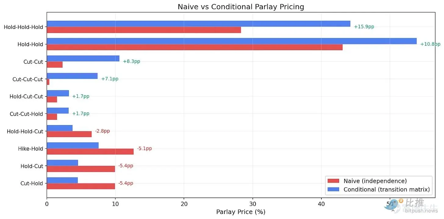
(Figure 5: Combinations involving consistent actions are systematically undervalued, while those involving directional switches are overvalued.)

Taking Polymarket's data as an example:

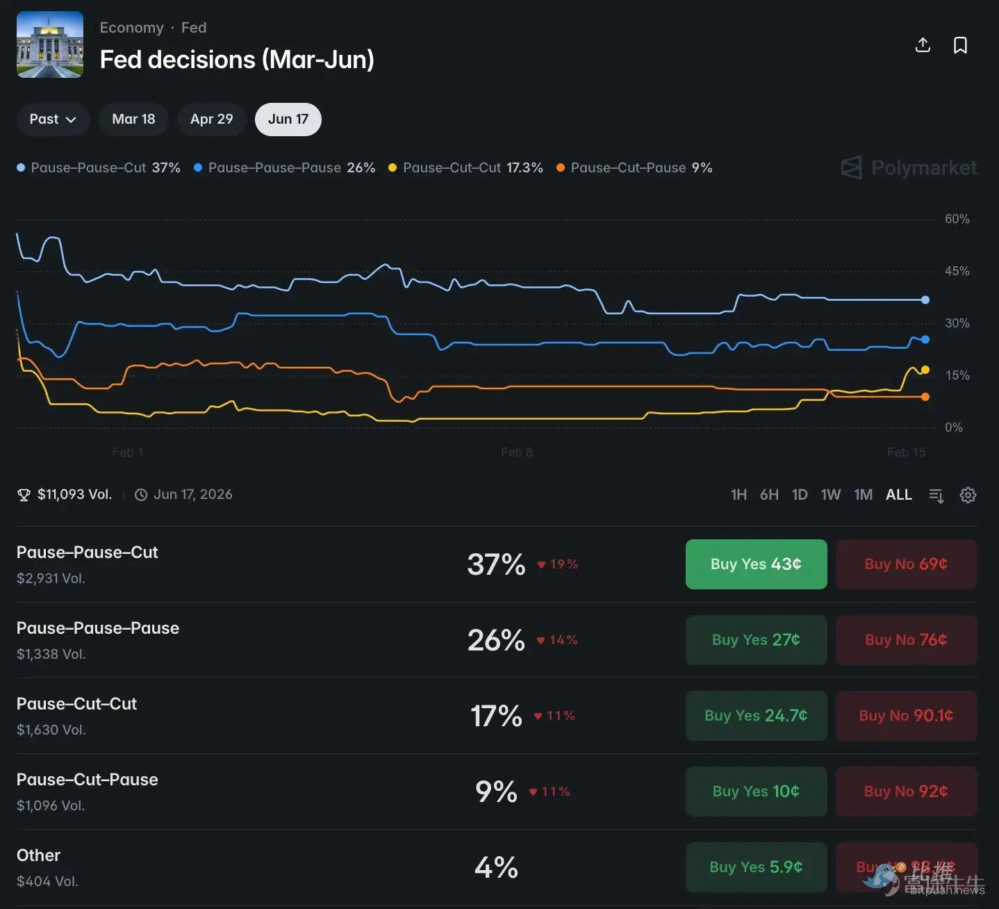
(Figure 6: Comparison of Polymarket odds distribution with actual probabilities)

Portfolio One: Hold – Hold – Hold (Severely Undervalued)

Initial model pricing: 93% (March) × 75% (April) × 38% (June) ≈ 26%

Conditional probability pricing: 87% × 87% × 87% ≈ 65.8%

Conclusion: The market is severely undervalued by up to 39 percentage points.

Portfolio Two: Hold – Hold – Rate Cut (Severely Overvalued)

Initial model pricing: 93% × 75% × 49% = 34.2%

Conditional probability pricing: 87% × 87% × 8.5% = 6.4%

Conclusion: The market prices this scenario at approximately 34%, while the actual probability is only 6.4%. Market prices are overestimated by more than five times.

I conducted a simple backtest. For every pair and every set of three consecutive Federal Reserve meetings since 1994, I placed a $100 bet if the adjusted price was higher than the market price (indicating undervaluation).

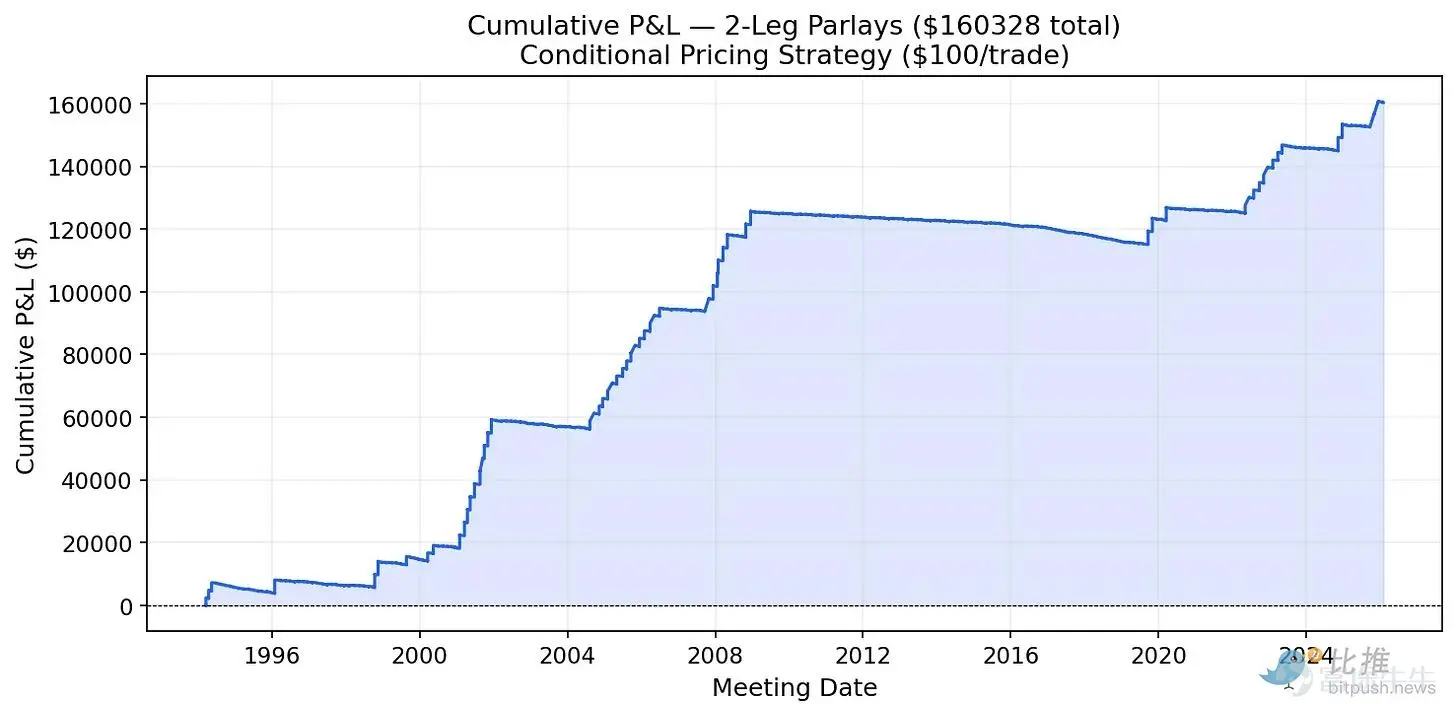
(Figure 7: Example of cumulative profit and loss for two consecutive bets)

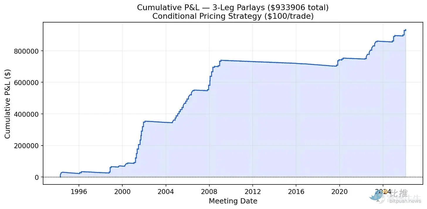
(Figure 8: Example of cumulative profit and loss for three consecutive bets)

Since 1994, betting $100 on each undervalued combination would have generated $169,000 in profits for two consecutive events and over $1 million for three consecutive events. The sharp rise in the profit curve corresponds to the Fed's easing cycles in 2001, 2008, 2020, and 2024-2025. During these cycles, repeated identical actions occurred consecutively, while the initial model consistently underestimated this continuity.

The 'step-like' pattern of the curve tells us that money is made during periods of sustained Fed action. However, the limitation is that there may not have been well-developed prediction markets in the 1990s to 2000s to execute these trades.

The Federal Reserve case is typical because of its abundant data and strong relevance. But the same framework applies to any correlated events:

Presidential candidate primaries: If a candidate wins in one state, his chances of winning in states with similar demographics will change.

Cryptocurrencies and macro/growth stocks: The movement of Bitcoin correlates with macro risk appetite. Betting on 'Bitcoin above X and Nasdaq above Y' has a value higher than the product of their independent probabilities, as they share common drivers.

In any case, the approach remains the same: examine historical data, measure the real connections between events, replace blind averages with better data, and compare it with market prices.

Prediction markets are still in their infancy. Most retail participants are still using the rudimentary method of 'simple multiplication and leaving it to fate' when pricing 'parlay bets.'

This framework requires knowledge of the specific context, but ultimately boils down to one question: Can the outcome of the first event tell you something about the next event? If it can, then the naive parlay pricing is wrong, and historical data will tell you exactly how much it’s off by.

The Federal Reserve's case study shows that this advantage is real and measurable. However, this principle is universally applicable. In any scenario where related events are priced as independent ones, there may be undiscovered opportunities.

The only question is whether you can see it and take action.

1345 Views